Data processing
This page aims to explain how to process data, from the raw file acquisition to the final rasters creation. It is divided into 6 steps as follow :

Note
The upcoming steps description is based on the demo dataset. This dataset contains a small data sample to have a fast processing.
This dataset aims to describe the process, but feel free to add you own dataset. Just keep in mind the format requirement at Step 2
Step 1 : Define your dataset name and folder
The first step is to define the name of your dataset. For the purpose of this tutorial, we will use the demo name.
Create or make sure that the folder demo folder exits :
Step 2 : Start you conda environment
Activate you conda environment as follow :
cd <your Topo-datagen folder>
conda activate topo-datagen
Step 3 : Data downloading and preprocessing
Objective : Prepare the data for the local and Cesium Ion processing.
There are 3 csv files under the demo folder. These files contain urls that for the following initial data:
File name |
Description |
Format |
Coordinate system |
Altitude |
|---|---|---|---|---|
surface3d.csv |
URLs for LIDAR data |
las |
EPSG:3857 |
Local altitude |
surface3d-raster.csv |
Digital surface model |
tif |
EPSG:3857 |
Ellipsoid height |
swissimage10.csv |
Orthophoto |
tif |
EPSG:3857 |
Run the follwing command to download the files and start the preprocessing :
export SCENE=demo

python scripts/preprocess_data.py $SCENE -dataDownload
Aternatively, if you have your own source files, you can create manually the following strucure:
and run the following command to start the preprocessing (needed only if you add your own file) :
export SCENE=demo

python scripts/preprocess_data.py $SCENE
Note
Here are the files formats requirements :
Folder name |
Description |
Format |
Coordinate system |
Altitude |
|---|---|---|---|---|
demo-surface3d |
LIDAR data |
las |
EPSG:3857 |
Local altitude |
demo-surface3d-raster |
Digital surface model |
tif |
EPSG:3857 |
Ellipsoid height |
demo-swissimage10 |
Orthophoto |
tif |
EPSG:3857 |
The data can be composed of one or many files. A merging process will be run anyway.
Step 4 : Data loading into Cesium Ion
Objective : Load the data into Cesium Ion and reference your token and AssetID
Load the file data_preprocess/demo/demo-surface3d-raster/mergedTIF-wgs84.tif into Cesium Ion
When uploading the .tif file, select the kind as raster terrain and choose base terrain as Cesium World Terrain, Meter and Ellipsoid height.

Compress the /data_preprocess/demo/demo-surface3d/ecef folder in .zip file and upload it as an point cloud.

Once uploaded, set the Point cloud location
Click on the pointcloud tiles
Click the Adjust Tileset Location button on the right top preview window of the 3D tile asset.

Click the Global Settings on the top left
Select the Terrain as ‘*-mergedTIF-wgs84’ we uploaded and click ‘Back to Assets’ to save the changes.

Copy the assetID of the point cloud
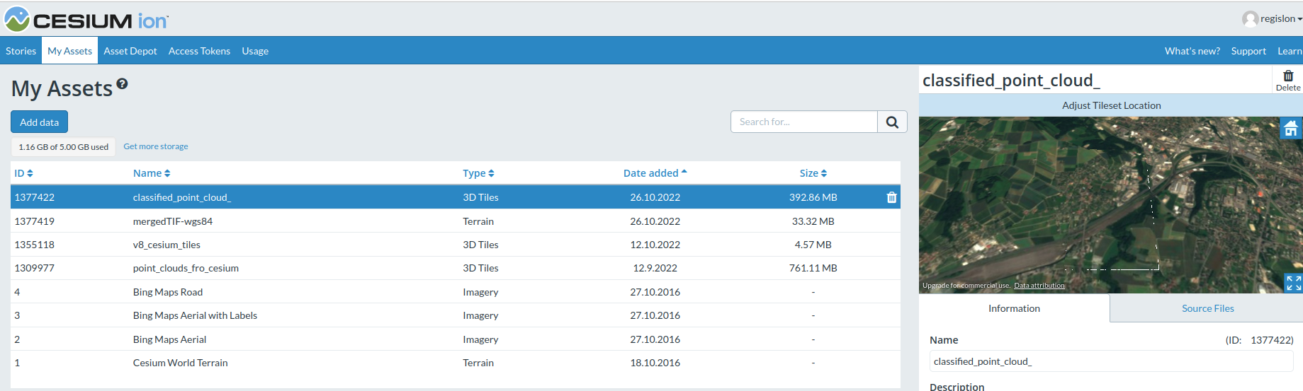
Copy your access_token. It can be accessed via Access Token besides ‘My Assets’ tab.

Paste the ID and token into the secret config file TOPO-DataGen-current-dev/scripts/.secrets.yaml
Step 5 : Data Processing
You can now start generating the synthetic images. In order to define the location of the poses, you can either use the position from the drone footage, or generate random positions (LHS).
Data Processing based on drone footages
Objectives : Create synthetic images based on given camera poses from real data collected by the DJI drone.
First download the drone footages from this link. Unzip the picture into a folder <your_drone_footages_folder> .
Run the following script:
export OUT_CESIUM_DIR=<your_cesium_folder>
export PHANTOM_DIR=<your_drone_footages_folder>
export SCENE=demo
export OUT_SYNTHETIC_SCENEMATCHING_DIR=scene-matching

python scripts/start_generate.py $OUT_SYNTHETIC_SCENEMATCHING_DIR $SCENE -matchPhantom $PHANTOM_DIR -cesiumhome $OUT_CESIUM_DIR
It creates synthetic images in the folder OUT_SYNTHETIC_SCENEMATCHING_DIR.
Data Processing based on random positions
Objectives : Create synthetic images based on random positions within the area (LHS - Latin hypercube sampling).
Configure the sampling boundary in script/presets/demo.json. The configuration parameter is of great significance for the redering of the synthetic images.
Change the latitude range to cover your area of interest
Change the longitude range to cover your area of interest
Make sure the height is about 100~200 meters above the ground of the area.
Once the Json presets is configured, run the following script :
export OUT_CESIUM_DIR=<your_cesium_folder>
export SCENE=demo
export OUT_SYNTHETIC_LHS_DIR=$SCENE-LHS
export PRESET=scripts/presets/demo.json

python scripts/start_generate.py $OUT_SYNTHETIC_LHS_DIR $SCENE -p $PRESET -cesiumhome $OUT_CESIUM_DIR
It creates sythetic images in the folder OUT_SYNTHETIC_LHS_DIR.
After the rendering is finished, we suggest running the helper scripts to clean the data and do some simple sanity check as follows:
export OUT_CESIUM_DIR=<your_cesium_folder>
export SCENE=demo
export OUT_SYNTHETIC_LHS_DIR=$SCENE-LHS
export LAS_DIR=$(pwd)/data_preprocess/$SCENE/****-surface3d/ecef-downsampled

python scripts/remove_outliers.py --input_path $OUT_CESIUM_DIR/$OUT_SYNTHETIC_LHS_DIR --las_path $LAS_DIR --save_backup
python scripts/tools/scan_npy_pointcloud.py --label_path $OUT_CESIUM_DIR/$OUT_SYNTHETIC_LHS_DIR --threshold 25
Necessary sanity check:
With the scan_npy_pointcloud.py, we would delete the synthetic image with reprojection error above 5 pixels. This may be caused by the fluctuation of the data steaming from the Ceisum Ion sever or local file loading issue. After that, run the following script to regenerate these images again until all the images look good and pass scan_npy_pointcloud check:
export OUT_CESIUM_DIR=<your_cesium_folder>
export SCENE=demo
export OUT_SYNTHETIC_LHS_DIR=$SCENE-LHS

python scripts/start_generate.py $OUT_SYNTHETIC_LHS_DIR $SCENE -cesiumhome $OUT_CESIUM_DIR
Step 6 : Retrieve semantics
Please note that we retrieve the pixel-wise semantic label based on the classified point cloud and scene coordinate. For each pixel in the frame, the closest matching point in the classified point cloud is identified and its class is used as the label.
We highly recommend to first clean the data (last step) to remove the outliers outside the boundary of the classified point cloud, as it improves the semantic recovery efficiency and quality.
export OUT_CESIUM_DIR=<your_cesium_folder>
export SCENE=demo
export OUT_SYNTHETIC_LHS_DIR=$OUT_CESIUM_DIR/$SCENE-LHS
export LAS_DIR=$(pwd)/data_preprocess/$SCENE/****-surface3d/ecef-downsampled
export SM_DIST_DIR=$OUT_SYNTHETIC_LHS_DIR-sm-dist

python scripts/semantics_recovery.py --input_path $OUT_SYNTHETIC_LHS_DIR --las_path $LAS_DIR --output_path_distance $SM_DIST_DIR
Note
CUDA device is preferred as the matrix computation could be much faster
Step 7 : Create raster
The last step consist of creating the different products (scene coordiantes, Semantics map, Euclidean depth, Surface normals, ORB keypoints).
export OUT_CESIUM_DIR=<your_cesium_folder>
export SCENE=demo
export OUT_SYNTHETIC_DIR=$SCENE-LHS
export RASTER_DIR=OUT_CESIUM_DIR/$SCENE-LHS-preview/

python scripts/export_data.py --pose_dir $OUT_CESIUM_DIR/$OUT_SYNTHETIC_DIR --out_dir $RASTER_DIR